This tutorial has two aims: 1. To provide an overview of the technique and application of Seismic Noise Interferometry (SNI); and 2. To act as a manual for the practical implementation of SNI by demonstrating the processing steps which I employ in my MRes research, and providing examples of results. This tutorial is available as PDF (click to download).

1. Background  

In seismology, the term "noise" refers to ground motion which is recorded in the absence of an identifiable source of seismic energy, such as an earthquake. At low frequencies, this ambient noise is caused primarily by the continuous interaction of oceanic surface waves ("swells") with the Earth's crust; which create two "microseismic peaks" which are observed globally. In most seismic applications steps are taken to remove ambient noise, as it acts to obscure other seismic signals which are traditionally used to infer information about the subsurface, such as the P-, S-, and surface waves generated by earthquakes.

In recent years however it has emerged that ambient noise is far from useless: it has been demonstrated theoretically and in practice that by applying the simple operation of cross-correlation to pairs of ambient noise records, made at different locations on the surface, useful information about the seismic properties of the subsurface can be obtained. This process is referred to as Seismic Noise Interferometry (SNI).

The potential usefulness of ambient noise was shown in a 2004 paper [Wapenaar], which demonstrated that, in any medium, the cross-correlation of recordings of a random wavefield would theoretically reproduce the seismogram that would have been recorded at one of the recorder locations if there had been an impulsive seismic source at the other; this result is often described in terms of a Greens function (see sect. 1.1 below): because oceanic noise becomes random when averaged over a sufficient time period, the possibility of reproducing interstation Greens functions by cross-correlating pairs of ambient noise records began to be studied.

Green's functions

For seismological applications, the Greens function (GF)

between any pair of locations on or within the Earth's

surface, completely describes the seismic energy

which would result at one in response to an

impulsive source at the other. In other words, the GF

describes what effect the medium between the two

points has on an implusive source of energy. Complete GFs

exist only theoretically, as recording limitations

always mean that some energy is not recordable;

however, the GF can reasonably be thought of as

 the seismogram which results

from some seismic source, such as an earthquake (fig.1).                                                                                                                                                                                                                                                                                                

Cross-correlation

Cross-correlation is an operation which measures the similarity of two waveforms in time. It does this by identifying the time lag (τ), the amount which one of the signals is shifted relative to the other, which makes the two most similar. C_a,b, the cross-correlation between two signals "a" and "b" is a function of the time lag between the two, and is commonly defined as:

                                             C_a,b (τ) = ∫ u(t,a)u(t-τ,b) dt

Where integration is performed over the time span of the records (which must be the same), and the first and second u terms represent the amplitude of a and b at times t and t-τ respectively. 

A peak at a time lag τ in the cross-correlation function (CCF) between two signals, which occurs when the sum of the product u(t,a)u(t-τ,b) is maximum, therefore indicates that the two waveforms are most similar when b is shifted by that amount. Hence, an auto-correlation (cross-correlation of a signal with itself) has a maximum at zero time lag.

A useful way to understand the ability of SNI to retrieve interstation GFs is that cross-correlation highlights interstation traveltimes of seismic waves. In the simplest case, a wave which has travelled between two stations will cause a similar seismic signal at each, but shifted in time: the CCF of these records will contain a peak at a time lag corresponding to the traveltime of the coherent energy between the two stations.

Cross-correlation is performed for positive and negative time lags, such that NCFs contain both positive ("causal") and negative ("acausal") parts. As a result, the empirical GFs which emerge on NCFs in fact contain information about waves travelling along the interstation path in both directions: if the order of cross-correlation is station A to station B, an NCF will contain information about the energy recorded at station B in response to an impulsive source at station A, in the causal part, and energy recorded at station A in response to an impulsive source at station B in the acausal part (fig.2). If noise sources are evenly distributed on both sides of the interstation path, the GF should be perfectly symmetrical, though in reality this is rarely the case, and NCFs are often not symmetrical, reflecting a stronger noise source in the direction of one of the stations (see section 2). 

In order to retrieve complete Greens functions, which contain the whole suite of seismic waves created by an impulsve source (fig. 1), the random sources in question must be equally distributed in the subsurface (Wapenaar (2004)). Oceanic noise does not satisfy this condition: oceanic waves strike the crust horizontally and close to the surface, and as such oceanic noise consists mostly of surface waves, which can only propagate parallel to the Earth's surface.

Despite this restriction, since the first successful application of the method in 2004 [Shapiro and Campillo] it has been consistently demonstrated, both theoretically and empirically, that energy corresponsing to the surface wave part of interstation Greens functions can be at least partially reconstructed using SNI. Furthermore, it has been shown that this surface wave energy can be used to infer useful information about the Earth's subsurface properties in much the same way as traditional earthquake records. SNI may be of particular use in the field of volcano seismology, as recent studies have shown that it allows the detection of very small variations in surface wave velocity, with a high temporal resolution on the order of days, and that trends in these variations may correlate with volcanic events (Brenguier et. al. (2008)).

SNI represents a powerful new tool in Geophysics, as it allows the creation of multiple, highly repeatable synthetic sources, using only the naturally occurring background seismic noise as a true source. That SNI does not require an earthquake source represents a major advantage over other methods. SNI is still in its infancy, and it is still not completely understood what factors affect the extent to which GFs can be reproduced using the method (Yao et, al. Tibet), however ...

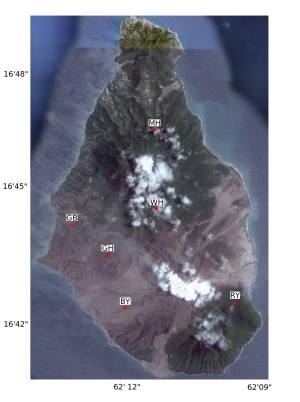
2. Current work - method

As part of my ongoing MRes research (due for submission in August 2010), I performed SNI using several weeks of continuous 3-component broadband seismic records from various stations in the Montserrat Broadband Network, Montserrat, West Indies (station map available here). Data were provided by the British Geological Survey in SEISAN format, and by the Montserrat Volcano Observatory in SEISLOG format.

Using the "wavetool" and "os9sei"programs included in the SEISAN analysis software, all data are first converted into SAC binary format, and all further processing conducted using the SAC processing software [reference].

All the following processing steps were automated using SAC macro scripting; the SAC commands used for each step are provided in bracketed italics. For a full explanation of the use of macros and each processing step I refer the reader to SAC's inbuilt help section, however all of the following processing steps are also easily implementable using most other common seismic analysis software.

Raw data pre-processing

The records are initially in 20 minute segments, which I concatenate into 1 day records (merge). Figure 1 shows a typical ambient noise signal, and figure 2 a full 24 hour record, both from the Montserrat broadband seismic network. Highly energetic events, such as those visisble in fig. 2, are undesirable in SNI as only the ambient noise signal provides the required coherent source wavefield; as such, various processing steps are applied to reduce the effect of larger amplitude events before cross-correlation is applied. 

1. The mean and trend are first removed from the data (rmean and rtrend respectively), which are then high pass filtered at 0.5Hz (hp). This frequency pass is expected to highlight scattered energy, which typically contains higher frequencies than the microseismic peaks which occur below 0.5Hz. 

2. Spectral whitening 

3. In order to down-weight the contribution of high-energy arrivals which could obscure the lower amplitude ambient noise signal, a "one-bit" normalisation is applied. This involves removing amplitude information completely, and keeping only the sign of the signal, by replacing each data point with either a 1 or -1. In the current work one-bit normalisation is achieved by dividing each 24h record (divf) by their absolute value (abs). 

Cross-correlation

The central step in the SNI method is the cross-correlation of pairs of ambient noise records. Processed 24h records are cross-correlated (cor) Reverse interstation paths were not computed (i.e. the cross-correlation BY-GB was performed but GB-BY was not), nor were reverse component pairs (BYZ-GBR was performed, but BYR-GBZ was not).

Secondly, for all station pairs with ZZ NCFs of sufficient quality, NCFs were computed for all further component pairs which correspond to Rayleigh wave particle motion: Vertical-Radial, and Radial-Radial. In addition, Vertical-Transverse NCFs were computed.

Horizontal records are provided in cartesian (NS-EW) coordinates, and it is therefore necessary to perform an appropriate rotatation in order to observe the non-vertical components of Rayleigh wave motion. This is achieved by rotating Z-N and Z-E NCFs (rotate) to the angle which minimises the energy on the Z-E NCFs: I define the Z-R NCFs  

It has recently been shown (Los Angeles paper) that in areas where oceanic noise is strongly directional, significant energy may be observed in the Greens tensor where none is expected (e.g. on Z-T NCFs). By rotating the records to the direction of the oceanic noise, it was shown that this effect could be partially removed. On Montserrat, noise can be reasonably expected to come primarily from an ESE direction (facing the Atlantic ocean) and indeed, by rotating records GB-RY and GH-RY to an angle of around 120°, the energy on the Z-T NCFs is minimised. 

Directionality of noise can therefore have two effects: 1. Non-symmetric NCFs; and 2. Incorrect particle motion (i.e. Z-T energy) on rotated station pairs. 

Finally the one day noise correlation functions (NCFs) are stacked over the whole 2 weeks (addf) to produce the master stacks. 

Assessment criteria

I assess the quality of the computed NCFs primarily on the basis of their signal to noise ratio (SNR), that is, the ratio of the amplitude of any emerging coherent signal to that of the incoherent background signal (fig. 5). A further assessment criterion used is the coherency between single day NCFs: while individual NCFs may stack coherently, day to say variation can be significant. It is commonplace in the literature (e.g. Brenguier et. al.) to perform running averages of days to weeks in order to stabilise the NCFs over time. 

Note the symmetricality of the peak energy arrival time

IMAGES: 15 day plots; Reference NCFs compared with single days. Spectrograms. 

Identifying surface wave energy

Particle motion

In order to test that the energy which emerges on the NCFs does in fact consist of Rayleigh waves, I examine the particle motion (PM) implied by the NCFs. In the vertical-radial plane, the PM of Rayleigh waves is retrograde elliptical in solids, this characteristic property should be observable in NCFs. Particle motion is computed (plotpm) for the vertical-vertical and (rotated) vertical-radial NCFs for each of the four high quality station pairs, as is PM between vertical-vertical and vertical-transverse NCF pairs in order to determine PM in the vertical-transverse plane, which should contain no surface wave energy. The time window over which to calculate PM is chosen according to where prominent energy occurs on both the Z-Z and Z-R NCFs. 

Figure 6 shows an example of a PM computation, for station pair BY-GB; the time period between -8 and -2.5 seconds is chosen as the PM window. PM is restricted mainly to the Z-R plane, where it exhibits the eliptical motion characteristic of Rayleigh waves. 

Velocity estimation

A crude estimate of the velocity of the (assumed) surface wave energy can be made using the interstation distance, and the time lag at which the amplitude of an NCF is maximum. By computing spectrograms ("spectrogram") (amplitude as a function of time and frequency), peak amplitude arrival times can be easily determined: for the Montserrat NCFs (fig. ), all coherent energy on NCFs is confined to time lags of less than 20 seconds, and peak energy occurs between 5 and 7seconds. Interstation distances are around 4-9 km, so these times indicate interstation velocities of between 0.8 and 1.3km/s, which are consistent with Rayleigh wave velocities in the shallow crust (reference). 

Station pair GB-MH (vertical component)